Some particular ADCP-observables
Acoustic Doppler current profilers ADCPs have three or four beams that are slanted towards the vertical at 15-30 degrees angles. They transmit and receive sound in a narrow band around a particular frequency. The reflection of the sound at suspended material, notably biological (zoo-)plankton, in a certain ‘range-gated’ volume determines the local velocity in all three Cartesian components, averaged over the beam spread over a range of known distances from the instrument. Below some less common observables are described using such instrumentation, in a moored fashion.
Direct estimates of turbulent fluxes
Turbulence estimates are difficult to make in the ocean. Most commonly a shipborne microstructure profiler is used, providing turbulence estimates from high-resolution shear measurements. This gives some insight in the spatial variability of turbulence, but has a rather poor resolution in time. Over the years, methods have been tried to use moored instruments to estimate turbulence with high temporal resolution. Perhaps the best method is using small-volume (~1 cm3) single point samplers of velocity in all three directions, but in order to resolve the large energy containing turbulent scales of up to 100 m one requires many of these along a mooring line which results in a rather expensive experimental set-up. With the advent of reliable ADCP’s an alternative was sought in estimating turbulent fluxes in the 19eighties. The method relies on the Reynolds decomposition of dynamic quantities (flow, temperature, …) in a ‘mean’ and a ‘fluctuating’ part. The mean of the cross-product of different fluctuating components will give a net flux that works on the mean quantity, provided that the fluctuating components are not in quadrature (as in linear waves, having zero cross-correlation). In practice however, the ocean does not show a spectral gap for a suitable decomposition between mean and fluctuating parts. Also, ADCP’s slanted beams require averaging over a relatively large horizontal area, although it is proven that one requires averaging of the statistics, not necessarily the current components. Given these caveats, the method is difficult to use in the open-ocean environment yielding some reliable momentum flux estimates in near-boundary flows mainly. Heat (buoyancy) flux estimates are even harder to make unambiguously, in a statistically confident sense, because of the matching of completely different sensor (techniques). In the past we have tried, with miscellaneous results.
Frontal passages
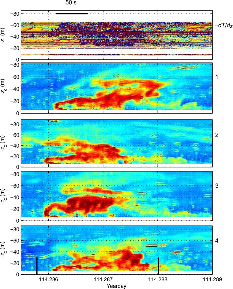 The ADCP’s backscatter or echo intensity data can be used as a primitive 3D directional antenna for observing turbulence processes, e.g. above sloping ocean bottoms. Although a single frequency ADCP cannot provide quantitatively reliable echo intensity data, the propagation direction and phase speed can be inferred, after some correction for the deformation of the signals due to slanted beams. It requires an ADCP fixed in space, e.g. mounted in a bottom lander. The observations may qualitatively back-up the 3D T-string mooring observations.
Deep plankton lunar motions
As known since the early days of acoustic profilers, ADCPs echo intensity can be used to qualitatively infer amounts of (mainly zoo-)plankton and to quantitatively estimate the plankton’s diurnal migration. This has been established not only for the photic zone, but also deeper in the ocean, even deeper than 1000 m where not a single photon of sunlight penetrates. After leaving ADCPs for more than one year at such depths it was observed that the records showed a strong monthly lunar periodicity. This is not related with the tidal spring-neap cycle, which is fortnightly, but entirely a modulation of the diurnal vertical plankton migration driven by and in phase with the moon: During full moon the plankton motion were most vigorous, at depths where no sunlight and certainly no moonlight ever penetrates.